Introduction to Transmission Lines
In low-frequency circuits, we often assume that wires have no length and no delay. As frequency increases, that assumption slowly breaks down. Voltage and current no longer appear the same everywhere along a conductor, and connections begin to behave like guided wave structures. At this point, they must be treated as transmission lines.
Transmission lines are central to RF, microwave, and high-speed digital design. They govern how efficiently power is delivered, how much signal is reflected, and how stable an amplifier, antenna, or matching network will be. Once their behavior is clear, many “mysterious” RF effects become intuitive and predictable.
1. When Does a Wire Behave Like a Transmission Line?
The threshold is set by the wavelength \( \lambda \) of the signal on the structure:
\[ \lambda = \frac{v_p}{f}, \quad v_p = \frac{c}{\sqrt{\varepsilon_\text{eff}}} \]
Here \( v_p \) is the phase velocity along the line, \( c \) is the speed of light in free space, and \( \varepsilon_\text{eff} \) captures the effect of the surrounding dielectric. As frequency or effective permittivity increases, the wavelength shrinks, and even physically short traces or cables can become electrically long.
A widely used guideline is: if the line length \( \ell \) is greater than about \( \lambda/10 \), then phase, delay, and reflection effects must be modeled using transmission line theory. Below that, lumped approximations may still work, but the margin rapidly disappears as \( \ell \) approaches \( \lambda/4 \) and beyond.
Example – 1 GHz Trace on a PCB
Consider a line on a substrate with effective permittivity \( \varepsilon_\text{eff} \approx 4 \). The phase velocity is approximately \( v_p \approx c/2 \), so the wavelength at 1 GHz is roughly \( \lambda \approx 15\ \text{cm} \). One-tenth of this is about 1.5 cm.
That means a 2–3 cm microstrip trace at 1 GHz is already in the transmission line regime. Ignoring impedance, reflections, and terminations at these dimensions can quickly lead to gain ripple, poor matching, or unstable behavior in RF circuits and antennas.
2. Basic Transmission Line Structure
Practical transmission lines come in many forms—coaxial cables, twisted pairs, microstrip lines, stripline, coplanar waveguides, and so on. Conceptually, however, they can all be viewed in the same way: a source drives energy into a structure with a characteristic impedance \( Z_0 \), and that structure delivers energy to a load \( Z_L \).
The electromagnetic fields are confined in and around the conductors. For circuit-level analysis, we replace this geometric complexity by a simpler model using \( Z_0 \), the propagation constant \( \gamma \), and the line length \( \ell \). These parameters are sufficient to capture reflections, standing waves, and power flow.
The simplest conceptual diagram shows a voltage source feeding a section of uniform line, which then terminates in a load. All the details of cross-section and dielectric are hidden inside the symbol for the transmission line.
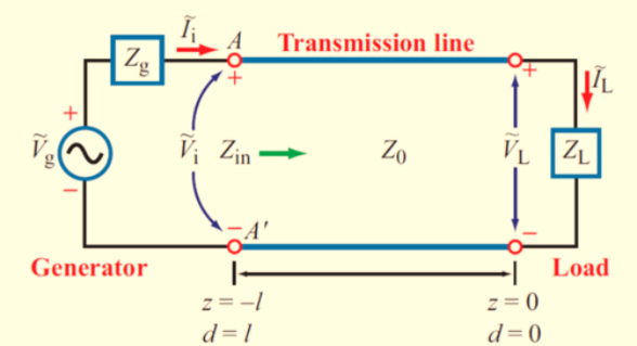
This compact representation is what most microwave texts use, and it is the basis for S-parameter blocks in simulators. Once the parameters of the line are known, the behavior of this three-block chain can be analyzed at any frequency of interest.
3. Distributed Model and Telegrapher’s Equations
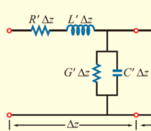
To connect geometry to circuit behavior, a uniform transmission line is modeled using distributed parameters. Over an infinitesimal section of length \( \Delta z \), the line is represented by series resistance \( R' \Delta z \) and inductance \( L' \Delta z \), along with shunt conductance \( G' \Delta z \) and capacitance \( C' \Delta z \) between the conductors.
Cascading many such sections and applying Kirchhoff’s laws leads to the Telegrapher’s Equations, which describe how voltage and current vary along the line:
\[ \frac{\partial V(z)}{\partial z} = - (R' + j\omega L')\, I(z) \] \[ \frac{\partial I(z)}{\partial z} = - (G' + j\omega C')\, V(z) \]
These coupled differential equations are the foundation of transmission line theory. From them, we obtain both the propagation constant \( \gamma = \sqrt{(R' + j\omega L')(G' + j\omega C')} \) and the characteristic impedance \( Z_0 \).
For many practical RF lines over moderate distances, losses are small enough that \( R' \ll \omega L' \) and \( G' \ll \omega C' \). In that case, the line behaves approximately as a lossless medium with:
\[ Z_0 \approx \sqrt{\frac{L'}{C'}}, \quad \gamma \approx j\beta \]
Once the distributed model is understood, it becomes easier to see how symmetric structures like coax or microstrip lead to specific values of \( L' \) and \( C' \), and therefore to standard impedances such as 50 Ω and 75 Ω in RF systems.
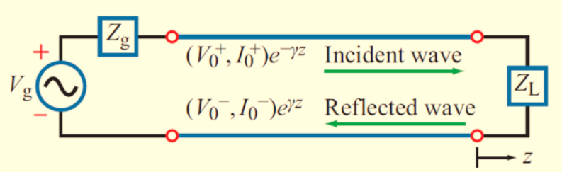
4. Voltage and Current Waves on a Transmission Line
Solving the Telegrapher’s Equations for a uniform line in sinusoidal steady state yields forward and backward traveling waves of voltage and current. The general solution can be written as:
\[ V(z) = V^+ e^{-\gamma z} + V^- e^{+\gamma z} \] \[ I(z) = \frac{V^+}{Z_0} e^{-\gamma z} - \frac{V^-}{Z_0} e^{+\gamma z} \]
Here \( V^+ \) is the amplitude of the wave launched from the source toward the load, and \( V^- \) is the amplitude of the wave reflected back from the load. The propagation constant \( \gamma = \alpha + j\beta \) incorporates both attenuation \( \alpha \) and phase constant \( \beta \).
In an ideal matched case with \( Z_L = Z_0 \), we have \( V^- = 0 \) and there is only a forward wave, gradually attenuated by loss. In mismatched cases, the reflected component interferes with the forward wave to create standing waves along the line.
5. Reflection Coefficient at the Load
The connection between the load impedance and the reflected wave is captured by the reflection coefficient at the load:
\[ \Gamma_L = \frac{V^-}{V^+}\Bigg|_{z=0} = \frac{Z_L - Z_0}{Z_L + Z_0} \]
The magnitude \( |\Gamma_L| \) tells what fraction of the wave amplitude is reflected, while the angle \( \angle \Gamma_L \) gives the phase of the reflected wave relative to the incident wave. Together, they determine the shape of the standing wave pattern, and how much power is delivered to the load.
Three classic special cases are particularly important:
- \( Z_L = Z_0 \) ⇒ \( \Gamma_L = 0 \): perfectly matched, no reflection.
- \( Z_L = 0 \) ⇒ \( \Gamma_L = -1 \): short circuit, full reflection with 180° phase shift.
- \( Z_L \to \infty \) ⇒ \( \Gamma_L = +1 \): open circuit, full reflection, no phase shift.
Example – 50 Ω Line with 100 Ω Load
Let \( Z_0 = 50\ \Omega \) and \( Z_L = 100\ \Omega \). The reflection coefficient is:
\[ \Gamma_L = \frac{100 - 50}{100 + 50} = \frac{50}{150} \approx 0.333 \]
About 33% of the incident voltage amplitude is reflected. The corresponding VSWR is:
\[ \text{VSWR} = \frac{1 + |\Gamma_L|}{1 - |\Gamma_L|} = \frac{1 + 0.333}{1 - 0.333} \approx \frac{1.333}{0.667} \approx 2 : 1 \]
A 2:1 VSWR still allows reasonable power transfer, but the standing waves are already noticeable. Tighter matching is often required in high-power or very sensitive systems.
6. Input Impedance of a Transmission Line
Once the load and line parameters are known, an important question is: what impedance does the line present at some distance away from the load? This is the input impedance \( Z_\text{in} \), which tells how the load “looks” when viewed through a length of transmission line.
For a uniform, lossless line of characteristic impedance \( Z_0 \), terminated in a load \( Z_L \) and of length \( \ell \), the input impedance at the beginning of the line is:
\[ Z_\text{in}(\ell) = Z_0 \frac{Z_L + j Z_0 \tan(\beta \ell)} {Z_0 + j Z_L \tan(\beta \ell)} \]
This expression shows how impedance transforms along the line as a function of its electrical length \( \beta \ell \). Even if the load is purely resistive, the input impedance can become complex-valued unless the line is very short or perfectly matched.
In practical design work, Smith charts or simulation tools are often used to visualize this transformation. However, keeping the analytic form in mind helps in quickly validating results and understanding the behavior of matching networks and stubs.
Example – 50 Ω Line, 100 Ω Load, Length λ/8
Assume a lossless line with \( Z_0 = 50\ \Omega \), load \( Z_L = 100\ \Omega \), and electrical length \( \beta \ell = \pi/4 \) (i.e., \( \ell = \lambda/8 \)).
\[ Z_\text{in} = 50 \cdot \frac{100 + j 50 \tan(\pi/4)}{50 + j 100 \tan(\pi/4)} = 50 \cdot \frac{100 + j 50}{50 + j 100} \]
The exact complex value can be computed numerically, but the key idea is that the impedance at the input has both real and reactive parts. As the line length changes, this point moves around the constant-\(|\Gamma|\) circle on a Smith chart, which is exactly how impedance matching with line sections is visualized.
7. Special Cases: Matched, Open, and Short-Circuited Lines
The general input impedance formula simplifies nicely for several important terminations. These cases appear repeatedly in stubs, resonators, and filters, and they are worth memorizing because they immediately suggest how a given line will behave.
\[ Z_\text{in}(\ell) = Z_0 \frac{Z_L + j Z_0 \tan(\beta \ell)} {Z_0 + j Z_L \tan(\beta \ell)} \]
7.1 Matched Line (\( Z_L = Z_0 \))
When the load is matched to the line, the expression collapses to:
\[ Z_\text{in}(\ell) = Z_0 \]
In this ideal case, the line appears as a pure resistance equal to its characteristic impedance, independent of length. No standing waves are formed, and all power launched into the line is ultimately absorbed by the load.
7.2 Open-Circuited Line (\( Z_L \to \infty \))
For an open circuit, the current at the load must be zero. The input impedance becomes:
\[ Z_\text{in}(\ell) = -j Z_0 \cot(\beta \ell) \]
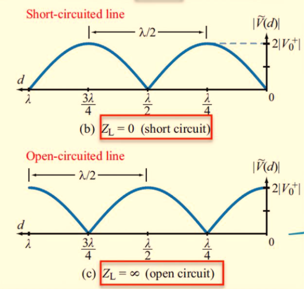
This impedance is purely reactive and alternates between capacitive and inductive as the line length changes. At lengths \( \ell = \lambda/4, 3\lambda/4, \dots \), the cotangent goes to zero and the input looks like a short circuit, even though the load end is open.
7.3 Short-Circuited Line (\( Z_L = 0 \))
For a short-circuited line, the voltage at the load must be zero. The input impedance is:
\[ Z_\text{in}(\ell) = j Z_0 \tan(\beta \ell) \]
Again, the impedance is purely reactive and cycles between inductive and capacitive with line length. At lengths \( \ell = \lambda/4, 3\lambda/4, \dots \), the tangent goes to infinity, and the input looks like an open circuit even though the load end is shorted.
Open and shorted stubs, cut to carefully chosen lengths, are therefore very useful as frequency-selective reactive components, especially at microwave frequencies where physical inductors and capacitors may be lossy or impractical.
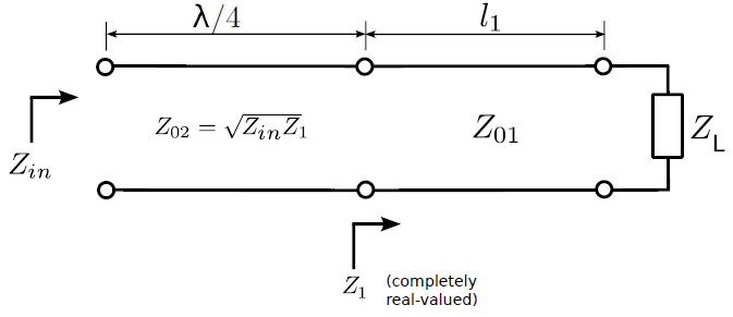
8. Quarter-Wave Transformer (λ/4 Matching Section)
A classic application of transmission lines is the quarter-wave transformer. A lossless line section of length \( \ell = \lambda/4 \) and characteristic impedance \( Z_1 \) can transform one real resistance into another, providing a simple, one-section matching network at a chosen frequency.
Consider a line of impedance \( Z_1 \) and length \( \ell = \lambda/4 \), placed between a line of impedance \( Z_0 \) and a purely real load \( R_L \). At \( \beta \ell = \pi/2 \), the input impedance is:
\[ Z_\text{in} = \frac{Z_1^2}{R_L} \]
For perfect matching, we require \( Z_\text{in} = Z_0 \), which leads to the familiar design rule:
\[ Z_1 = \sqrt{Z_0 R_L} \]
A single λ/4 section with this impedance will ideally match \( Z_0 \) to \( R_L \) at the design frequency. The bandwidth of the match depends on how different \( Z_0 \) and \( R_L \) are, and multi-section transformers can be used when a wider match is required.
Example – Matching 25 Ω to 100 Ω
Suppose a 100 Ω system must efficiently deliver power to a 25 Ω load at a particular frequency. Using a quarter-wave transformer, the required characteristic impedance is:
\[ Z_1 = \sqrt{Z_0 R_L} = \sqrt{100 \times 25} = 50\ \Omega \]
A λ/4 section of 50 Ω line at the design frequency is inserted between the 100 Ω side and the 25 Ω load. At that frequency, the combination is perfectly matched, and reflections are ideally eliminated. Away from that frequency, the match gradually degrades, which motivates multi-section matching networks for broadband applications.
9. Standing Waves and VSWR
When both incident and reflected waves are present, their superposition along the line produces a standing wave pattern. At some points, voltage adds constructively and reaches a maximum; at others, it cancels partially and reaches a minimum. The ratio of these extremes defines the Voltage Standing Wave Ratio (VSWR).
Let \( V_\text{max} \) and \( V_\text{min} \) denote the maximum and minimum voltage magnitudes along the line. Then:
\[ \text{VSWR} = \frac{V_\text{max}}{V_\text{min}} = \frac{1 + |\Gamma_L|}{1 - |\Gamma_L|} \]
A perfectly matched line has \( |\Gamma_L| = 0 \) and VSWR = 1, meaning the voltage amplitude is constant along the line. As \( |\Gamma_L| \) increases toward 1, the standing wave becomes more pronounced and VSWR grows toward infinity, indicating severe mismatch.
Instruments such as directional couplers and VSWR meters effectively measure \( |\Gamma| \) and present it as VSWR or return loss, providing a direct view of how well an antenna or load is matched to its feeding line.
10. Power Flow and Mismatch Loss
Reflection not only distorts the voltage and current distribution, it also reduces the net power delivered to the load. If \( P_\text{inc} \) is the incident power, the reflected power is \( P_\text{ref} = |\Gamma_L|^2 P_\text{inc} \), and the power actually delivered to the load is:
\[ P_\text{del} = P_\text{inc} - P_\text{ref} = P_\text{inc} (1 - |\Gamma_L|^2) \]
This relation is often expressed in terms of mismatch loss in decibels. For example, when \( |\Gamma_L| = 0.333 \) (VSWR ≈ 2:1), only about \( 1 - 0.333^2 \approx 89\% \) of the incident power reaches the load, and roughly 11% is reflected. Depending on the system, this may or may not be acceptable.
At very high power levels or in sensitive low-noise applications, even modest mismatch can be problematic, driving the need for precision matching networks and careful transmission line design from the source all the way to the antenna.
This introduction has built a complete, interconnected picture of transmission lines: when simple wires must be treated as lines, how distributed parameters lead to the Telegrapher’s Equations, how forward and reflected waves arise, how reflection coefficient and VSWR quantify mismatch, and how input impedance depends on load and line length.
Special cases such as matched, open, and short-circuited lines naturally lead to useful structures like stubs and quarter-wave transformers. These ideas are the backbone of many RF and microwave components, from antenna feeds to filters and matching networks.