Microstrip Patch Antenna Design: Theory, Equations & Calculator

This project presents the complete design workflow of a rectangular microstrip patch antenna using classical transmission-line and cavity models. Starting from the desired resonant frequency \( f_r \), the post derives and applies closed-form equations for patch width \( W \), effective permittivity \( \epsilon_{\text{eff}} \), length extension \( \Delta L \), and actual patch length \( L \). The theoretical formulation is followed by an interactive calculator implemented in JavaScript, enabling students to quickly obtain patch dimensions or estimate the resonant frequency for a given geometry. The post concludes with simulation guidelines for CST Microwave Studio and a curated list of standard references (Balanis, Garg, Pozar, Kumar & Ray) for deeper study.

Keywords: Microstrip Patch Antenna, Rectangular Patch, Transmission-Line Model, Effective Permittivity, CST Simulation, RFInside Project

1. Introduction

Microstrip patch antennas have become the workhorse of modern RF and wireless systems because they are compact, lightweight, planar, and compatible with low-cost PCB fabrication. They are used in WLAN, GNSS, LTE, 5G sub-6 GHz, automotive, and IoT applications where profile, cost, and integration are critical.

The most basic configuration is the rectangular microstrip patch antenna, consisting of a metal patch on a dielectric substrate backed by a ground plane. For the dominant mode, the structure can be modeled as a resonant cavity with fringing fields at the radiating edges. This project focuses on the design of such a rectangular patch operating in the fundamental \( \text{TM}_{10} \) mode.

2. Microstrip Patch Antenna Fundamentals

2.1 Geometry and Substrate Parameters

A rectangular microstrip patch antenna is characterized by:

• Patch width: \( W \)
• Patch length: \( L \)
• Substrate relative permittivity: \( \epsilon_r \)
• Substrate thickness: \( h \)
• Ground plane dimensions: usually \( L_g \approx 6h + L \), \( W_g \approx 6h + W \)

For most practical designs, conductor thickness is small compared to \( h \) and is neglected in first-order calculations. The choice of \( \epsilon_r \) and \( h \) affects bandwidth, efficiency, and size:

• Low \( \epsilon_r \) (e.g., 2.2–3.0): larger size, better efficiency and bandwidth.
• Higher \( \epsilon_r \) (e.g., FR-4, \( \epsilon_r \approx 4.3\text{–}4.6 \)): smaller size, but radiation efficiency may decrease.

2.2 Dominant Mode and Resonant Behavior

For the rectangular patch, the dominant resonant mode is \( \text{TM}_{10} \), where the field variation is primarily along the patch length \( L \) and approximately uniform along the width \( W \). The resonant frequency for this mode can be approximated (using the cavity model) as:

\( f_r \approx \frac{c}{2 L_{\text{eff}} \sqrt{\epsilon_{\text{eff}}}} \)

where \( c \) is the speed of light, \( L_{\text{eff}} \) is the effective length including fringing, and \( \epsilon_{\text{eff}} \) is the effective dielectric constant.

2.3 Effective Dielectric Constant

Because the fields are partly in the dielectric and partly in the air, the structure does not behave like a pure dielectric-filled cavity. Instead, we define an effective permittivity:

\( \epsilon_{\text{eff}} = \frac{\epsilon_r + 1}{2} + \frac{\epsilon_r - 1}{2}\left(1 + 12\frac{h}{W}\right)^{-1/2} \)

This parameter is used to compute the guided wavelength and effective electrical length of the patch.

3. Design Equations for Rectangular Patch

3.1 Patch Width \( W \)

The width is often chosen to optimize radiation efficiency and bandwidth. A commonly used expression is:

\( W = \frac{c}{2 f_r} \sqrt{\frac{2}{\epsilon_r + 1}} \)

where: \( c \) = speed of light, \( f_r \) = desired resonant frequency, \( \epsilon_r \) = substrate relative permittivity.

3.2 Effective Permittivity \( \epsilon_{\text{eff}} \)

Using the width \( W \) from the previous step and the substrate height \( h \), we compute \( \epsilon_{\text{eff}} \) from:

\( \epsilon_{\text{eff}} = \frac{\epsilon_r + 1}{2} + \frac{\epsilon_r - 1}{2}\left(1 + 12\frac{h}{W}\right)^{-1/2} \)

3.3 Fringing and Length Extension \( \Delta L \)

Due to fringing at the open-circuit radiating edges, the effective electrical length is slightly larger than the physical length. The empirical length extension on each side is:

\( \Delta L = 0.412 h \frac{(\epsilon_{\text{eff}} + 0.3)(W/h + 0.264)}{(\epsilon_{\text{eff}} - 0.258)(W/h + 0.8)} \)

3.4 Effective Length and Actual Length \( L_{\text{eff}}, L \)

The effective resonant length is given by:

\( L_{\text{eff}} = \frac{c}{2 f_r \sqrt{\epsilon_{\text{eff}}}} \)

and the actual physical patch length is:

\( L = L_{\text{eff}} - 2\Delta L \)

3.5 Reverse Calculation: Resonant Frequency from Geometry

If the patch dimensions are already chosen (e.g., from a PCB layout), we can estimate the resonant frequency:

1. Compute \( \epsilon_{\text{eff}} \) using the given \( W, h, \epsilon_r \).
2. Compute \( \Delta L \) using the fringing formula.
3. Obtain \( L_{\text{eff}} = L + 2\Delta L \).
4. Compute resonant frequency:
   \( f_r = \frac{c}{2 L_{\text{eff}} \sqrt{\epsilon_{\text{eff}}}} \).

4. Step-by-Step Design Workflow

A concise workflow to design a rectangular microstrip patch antenna:

1. Specify target frequency \( f_r \) and application (e.g., 2.45 GHz ISM band).
2. Select substrate material (e.g., FR-4, Rogers) with desired \( \epsilon_r \) and thickness \( h \).
3. Compute patch width \( W \) from the width formula.
4. Determine \( \epsilon_{\text{eff}} \) and length extension \( \Delta L \).
5. Compute patch length \( L \) from \( L_{\text{eff}} - 2\Delta L \).
6. Choose a suitable feed technique (coaxial probe, inset microstrip, proximity feed).
7. Create the geometry in CST Microwave Studio with a sufficiently large ground plane.
8. Set up ports, boundaries, and frequency sweep; observe \( S_{11} \), resonant frequency, and bandwidth.
9. Fine-tune \( L \), feed position, or inset depth to match the desired input impedance (typically 50 Ω).

5. Interactive Patch Antenna Calculators

The following calculators implement the standard closed-form equations discussed above. They allow quick estimation of patch dimensions for a given resonant frequency and vice versa. These tools are intended for preliminary design; final dimensions should always be validated with full-wave EM simulation.

5.1 Calculator A – Patch Dimensions from Resonant Frequency

5.2 Calculator B – Resonant Frequency from Patch Dimensions

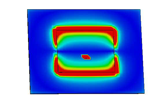
6. CST Simulation and Result Interpretation

Once the dimensions are finalized, the design must be validated using a full-wave EM simulator such as CST Microwave Studio (or HFSS, FEKO, etc.). In CST:

• Create a 3D model with patch, substrate, and ground plane.
• Assign appropriate materials (e.g., FR-4 with \( \epsilon_r \approx 4.4 \)).
• Define a discrete port or waveguide port depending on feed configuration.
• Set frequency range around the target \( f_r \) (e.g., 2–3 GHz for a 2.45 GHz design).
• Run a frequency-domain or time-domain solver to obtain \( S_{11} \), input impedance, and radiation pattern.

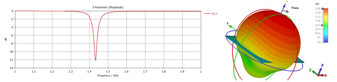
Typical expectations for a well-designed rectangular patch:

• Return loss \( S_{11} \leq -10 \) dB at the target frequency.
• VSWR close to 1:1–1.5:1 around resonance.
• Broadside radiation with gain typically in the range of 2–8 dBi (depending on substrate and size).
• Reasonable bandwidth (2–5% for thin, high-\( \epsilon_r \) substrates; higher for thicker, low-\( \epsilon_r \) substrates).

7. Downloadable Project Files (Python + CST)

To make this microstrip patch antenna project directly reproducible, we provide a consolidated ZIP archive containing:

• Python script for patch dimension and frequency calculation.
• CST Microwave Studio model with parameterized \( W, L, h, \epsilon_r \).
• A short readme explaining how to modify parameters and re-run simulations.

Download Microstrip Patch Antenna Project (ZIP)

8. References for Further Reading

• Balanis, C. A. (2016). Antenna Theory: Analysis and Design (4th ed.). Wiley.
• Garg, R., Bhartia, P., Bahl, I., & Ittipiboon, A. (2001). Microstrip Antenna Design Handbook. Artech House.
• Pozar, D. M. (2011). Microwave Engineering (4th ed.). Wiley.
• Kumar, G., & Ray, K. P. (2003). Broadband Microstrip Antennas. Artech House.
• Ramesh, G., et al. (various). Journal and conference papers on microstrip patch antenna enhancements (slots, stacked patches, and bandwidth improvement).