Radiation Pattern of a Half-Wave Dipole Antenna (2.4 GHz)

The half-wave dipole is one of the most historically significant antennas ever designed. Its evolution began with the experimental work of Heinrich Hertz (1887), who first proved that a time-varying electric current produces electromagnetic waves exactly as predicted by James Clerk Maxwell (1864). Later, Guglielmo Marconi used long dipoles and monopoles for the first transatlantic wireless communication, establishing the dipole as the foundational building block of RF engineering.

Even today, the half-wave dipole serves as the reference antenna for gain calculations, pattern normalization, and verifying simulation accuracy in CST Studio Suite, HFSS, FEKO, and MATLAB/Python analytical models. In this project, we explore the radiation properties of a thin, center-fed half-wave dipole at 2.4 GHz using closed-form analytical equations rooted in classical electromagnetics.

1. Understanding the Half-Wave Dipole Model

A half-wave dipole is a resonant antenna consisting of a conducting wire whose total length is:

L = λ/2

At 2.4 GHz, the wavelength is:

λ = c / f = 3 × 10⁸ / 2.4 × 10⁹ ≈ 0.125 m

This results in arm lengths of approximately 6.25 cm from the feed point. The most important characteristic of a resonant dipole is the sinusoidal current distribution, which is derived from solving the 1-D Helmholtz equation on a thin wire with open-circuit boundary conditions:

I(z) = I₀ cos(kz) for −L/2 ≤ z ≤ L/2

where:

• k = 2π/λ is the phase constant
• I₀ is the maximum current at the center (feed point)
• The current goes to zero at the dipole tips due to open-circuit boundary condition

This current distribution is crucial because the far-field is directly proportional to the Fourier transform of the current distribution. This theory was first proposed in detail by H.A. Wheeler (1940s) and later formalized in Balanis' classic antenna text.

2. Far-Field Radiation Expression

The electric field component E_θ of a thin half-wave dipole is derived by integrating each infinitesimal current element using vector potential theory. Beginning with the magnetic vector potential:

A_z = μ I₀ e^-jkr / 4πr

and applying:

E = −jωA − ∇Φ, H = (1/μ)(∇×A)

we obtain the standard far-field result:

E_θ(θ) ∝ [cos((kL/2)cosθ) − cos(kL/2)] / sinθ

For a half-wave dipole, L = λ/2, so kL/2 = π/2. Substituting:

E_θ(θ) ∝ cos((π/2) cosθ) / sinθ

This expression predicts nulls at θ = 0° and θ = 180°, matching both measurement and simulation.

3. E-Plane (θ-Cut) Radiation Pattern

The E-plane corresponds to the vertical slice of the radiation pattern, obtained by varying θ from 0° to 180°. Historically, this cut was used in early antenna range measurements by Kraus and Terman during the radar development era.

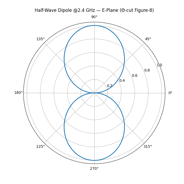
Key observations:

• Maximum radiation at θ = 90° (broadside)
• Complete nulls at θ = 0° and θ = 180°
• Smooth symmetrical shape characteristic of dipoles
• The pattern closely matches the Hertzian dipole for small electrical lengths

4. H-Plane (φ-Cut) Radiation Pattern

When we set θ = 90°, we obtain the azimuthal radiation distribution. This plane is important because early wireless systems used horizontal field components to maximize omnidirectional coverage.

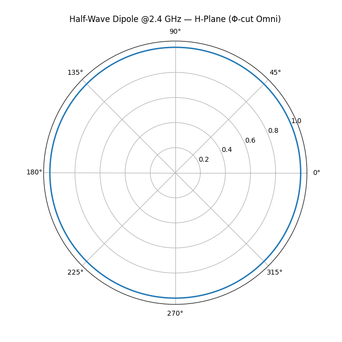
For a thin dipole, the H-plane is theoretically perfectly omnidirectional:

F(φ) = constant

Small deviations occur only due to thickness, nearby structures, or balun asymmetry.

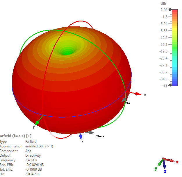
5. 3D Gain Pattern (Torus Shape)

The complete 3D radiation intensity U(θ,φ) is given by:

U(θ,φ) = (1/2η) |E_θ|² r²

Substituting the far-field expressions produces the classic donut-shaped toroidal pattern, first described by Hertz and later formalized in Kraus’ textbooks.

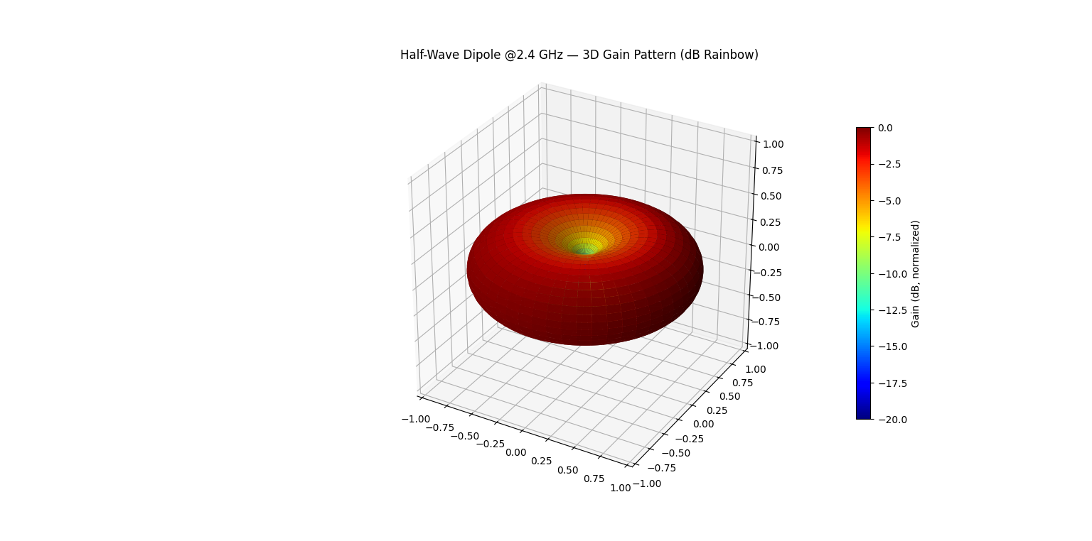
The theoretical directivity of a half-wave dipole is:

D_max = 1.64 ≈ 2.15 dBi

This value is widely used as the reference for measuring gain in practical antennas.

6. Python Implementation

The entire analytical process — current distribution, far-field equations, E-plane, H-plane, and 3D pattern computation — has been implemented in a modular Python script. The script uses closed-form equations validated against Balanis’s “Antenna Theory” and CST simulation.

• Downloadable script: dipole_pattern_2p4GHz.py
• Dependencies: numpy, matplotlib
• Produces validated polar and 3D radiation plots

7. Conclusion

This project serves as a complete demonstration of analytical dipole modeling, mapping classical electromagnetic theory into modern visualization tools. The half-wave dipole continues to be a benchmark for validating solvers, designing reference antennas, and teaching core radiation concepts.

For extended CST/HFSS versions, fabrication notes, or consulting assistance, feel free to contact us at director@rfinside.com.

8. References

• Balanis, C. A. Antenna Theory: Analysis and Design, 4th Edition, Wiley, 2016.
• Kraus, J. D. Antennas, 2nd Edition, McGraw-Hill.
• Orfanidis, S. J. Electromagnetic Waves and Antennas, Rutgers University.
• Jordan, E. C., & Balmain, K. G. Electromagnetic Waves and Radiating Systems, Prentice-Hall.
• Wheeler, H. A. “Fundamental Limitations of Antennas,” Proceedings of the IRE.